This page has been moved to our support documentation website.
See https://docs.vpixx.com/vocal/gamma-correct-the-luminance-of-a-display
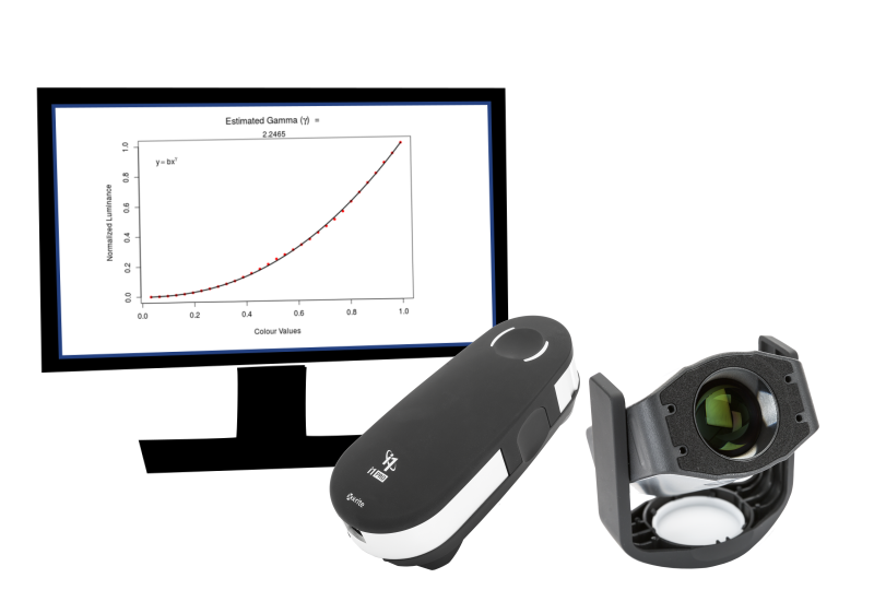
Gamma-Correct the Luminance of a Display
Sample the luminance of any display using an X-Rite photometer or colorimeter. Calculate the gamma value that characterizes the non-linearity of your display. Generate and apply the gamma-correction color lookup table that will linearize its luminance.
Contributed by:
Dr. Sophie Kenny, VPixx Technologies
Date published:
May 15, 2020