Download supplementary materials:


Download

Questions can be sent to: [email protected]

Overview

This project serves as an introduction to the TRACKPixx3 2 kHz binocular eye tracker and its output. It is geared towards new users of the TRACKPixx3 and those interested in learning more about the device.

We will start with a general explanation of TRACKPixx3 functionality, and discuss the format of the tracking data it provides. Next, we will go through a step-by-step implementation of a single-trial free image viewing task in MATLAB/Psychtoolbox. Finally, we’ll do some basic plotting of our gaze data, overlaid onto the viewed image.

For those wishing to follow along in MATLAB, the full code, supplementary material and some sample data can be downloaded from the side bar. You will need to have VPixx software tools installed, and your Psychtoolbox’s Datapixx.mex file should be updated with the one provided by the software install. For more details on installing our toolbox, see our installation guide. 

Principles of TRACKPixx3 operation

The TRACKPixx3 is a passive infrared binocular eye tracker. The device consists of an infrared LED lamp and a high-speed camera with a detachable lens. These components are mounted on an adjustable metal bracket, and positioned below your experiment display. 

Example TRACKPixx3 (tabletop version)

During data collection, the lamp bathes the participant’s face and eyes in non-visible infrared light, which the camera records. An image-processing algorithm determines the shape of the pupil and locates its center. It also identifies the corneal reflection, a bright spot created by the infrared light reflecting off the front surface of the eye.

VPixx hardware computes the vector between the pupil center and corneal reflection, which we call the pupil-corneal vector. This vector is used as the basis for determining where the participant is looking on the screen. 

The TRACKPixx3 detects the pupil shape and center, as well as the corneal reflection.

In order to interpret this vector properly, the TRACKPixx must have a notion of how this vector changes as a function of where your participant is looking on the screen. This relationship depends on a lot of external factors, like the size of your participant’s eyes, the position of their head, the size of the screen, the type of camera lens, and so on.

For this reason, before any eye tracking session begins you must perform a calibration procedure, to build up a model of your specific participant’s pupil-corneal vector dynamics. We will cover how to run a calibration procedure later in this project. 

The pigment of your iris looks different under infrared light. Dark brown eyes reflect more infrared light, which shows up as a light-coloured iris in the eye tracker video feed. Pale blue or green eyes absorb more infrared light, making them appear darker in the camera view. 

The TRACKPixx3 is connected to your computer via a DATAPixx3 video I/O hub. This hub also acts as an intermediary between your computer and stimulus display. It can optionally send a copy of your graphics card output to a second, “console” display. The console can be used by the experimenter to track progress, and is particularly useful if the experimenter is in another room, or cannot see the stimulus display easily.

The console also displays a live feed of the eye tracker in the top corner of the screen.

For more details on how to set up your TRACKPixx3 for the first time, please consult the installation guide that was included with your purchase. Installation guides can also be found in our online library.

Typical layout of a TRACKPixx3 tabletop setup

The DATAPixx3 I/O hub may also be connected to other peripherals. It can send and receive digital signals on two DB25 ports, enabling experimenters to log outgoing and incoming data on the same clock as eye tracking data. It can also send out analog eye position data via a third DB25 port, which may be connected to a recording rig like an EEG system. A DATAPixx3 “Full” unit can also play and record audio, and send and receive analog signals other than eye data.

The TRACKPixx3 buffer

During recording, eye tracking data are stored in a buffer in the DATAPixx3’s onboard memory at a rate of 2 kHz, or 2000 samples per second. Data are formatted as an m x 20 array, where m corresponds to the number of samples recorded.

The table below explains each of these columns of data. It is important to note that in VPixx eye tracking convention, right and left eyes correspond to the eyes as they appear on the console feed. In tabletop and MEG setups, this view is typically the inverse of the participant’s first-person perspective. In MRI setups with a vertical mirror, the view is consistent with first-person perspective. 

If you are unsure of which eye is labelled “right” and “left”, you can test this by covering an eye during tracking and checking the console view to see which eye is obscured.

TRACKPixx3 Buffer Contents
ColNameUnitsDescription
1Time tagsecondsTime, in seconds, since the DATAPixx3 was last turned on. Uses the same clock as all other I/O on the DATAPixx3 for easy synchronization.
2Left Eye xpixelsx screen coordinate, in pixels, corresponding to the calibrated x position of the left eye. Uses a Cartesian system where (0,0) corresponds to the center of the display.
3Left Eye ypixelsy screen coordinate, in pixels, corresponding to the calibrated y position of the left eye. Uses a Cartesian system where (0,0) corresponds to the center of the display.
4Left Eye Pupil DiameterpixelsThe diameter of the left pupil. The pupil is mapped as an ellipse; the diameter always reflects the major (longest) axis of this ellipse.
5Right Eye xpixelsx screen coordinate corresponding to the calibrated x position of the right eye. Uses a Cartesian system where (0,0) corresponds to the center of the display.
6Right Eye ypixelsy screen coordinate corresponding to the calibrated y position of the right eye. Uses a Cartesian system where (0,0) corresponds to the center of the display.
7Right Eye Pupil DiameterpixelsThe diameter of the right pupil. The pupil is mapped as an ellipse; the diameter always reflects the major (longest) axis of this ellipse.
8Digital InputintegerAn integer value which represents the 24-bit digital input to the DATAPixx3. This value will change in response to button box presses, incoming triggers, and any other input coming in from the Digital In port.
9Left Eye Blinkboolean0 if the left eye is open, 1 if the left eye is closed.
10Right Eye Blinkboolean0 if the right eye is open, 1 if the right eye is closed.
11Digital OutputintegerAn integer value which represents the 24-bit digital output being sent from the DATAPixx3. This value will change in response to outgoing triggers, e.g. from the DOut schedule or Pixel Mode.
12Left Eye FixationbooleanDefault 0, changes to 1 if the conditions for a left eye fixation event are met. By default, the fixation flag raises when the eye has moved less than 2500 pixels/second for the last 25 consecutive frames. These default thresholds can be changed by the user.
13Right Eye FixationbooleanDefault 0, changes to 1 if the conditions for a right eye fixation event are met. By default, the fixation flag raises when the eye has moved less than 2500 pixels/second for the last 25 consecutive frames. These default thresholds can be changed by the user.
14Left Eye SaccadebooleanDefault 0, changes to 1 if the conditions for a left eye saccade are met. By default, the saccade flag raises when the eye has moved more than 10,000 pixels/second for the last 10 consecutive frames. These default thresholds can be changed by the user.
15Right Eye SaccadebooleanDefault 0, changes to 1 if the conditions for a right eye saccade are met. By default, the saccade flag raises when the eye has moved more than 10,000 pixels/second for the last 10 consecutive frames. These default thresholds can be changed by the user.
16Message codeimplemented in future release
17Left Eye Raw xpixelsx value of the left eye pupil-corneal vector
18Left Eye Raw ypixelsy value of the left eye pupil-corneal vector
19Right Eye Raw xpixelsx value of the right eye pupil-corneal vector
20Right Eye Raw ypixelsy value of the right eye pupil-corneal vector

Gaze and pupil data that are missing due to tracking loss return as NaN (Not a Number). Tracking is lost when the participant blinks or looks away from display.

High-level control of recording can be done with PyPixx software utility. In PyPixx, recording is controlled by toggling on the “Record Eye Tracking Data” in the Demo > TRACKPixx widget. When recording ends, data are automatically imported and saved to a .csv file on your computer. 

Calibration and recording can be performed via PyPixx

For low level control, recording can be managed in MATLAB or Python via a TRACKPixx schedule. Buffer data can then be read directly into either program as a floating-point data array.  

With MATLAB and Python, it is possible to query buffer contents during recording. For example, users can get the current eye position, or check whether the participant is fixating. For a full list of TRACKPixx functions in Python, check the toolbox documentation for Python. For MATLAB, simply type ‘Datapixx’ in the command line for a full list of functions.

The DATAPixx3 internal memory can store roughly an hour of eye tracking data before it loops back to the beginning of the buffer and overwrites data. If you are using several buffers, the available memory for eye data will shrink accordingly.

We recommend that long experiments regularly import TRACKPixx3 data from the buffer (e.g., between trials or experiment blocks) to avoid overwriting data.

A simple free viewing task in MATLAB

To demonstrate the general strategy for using the TRACKPixx3, we will program a short free viewing task. In this task, participants are given 10 seconds to examine a painting displayed on the screen. We record eye position data and then import it from the buffer, and plot gaze paths for the left and right eyes superimposed over the painting itself. 

In this section we will go step-by-step through creating and running this task. To follow along with the code in MATLAB, download the supplementary materials available in the left-hand menu.  These materials include sample buffer data and a copy of the displayed painting, Renoir’s Lise in a White Shawl

Below is the plotted sample data, which shows a characteristic pattern of focusing on facial features. 

The original image, and a copy with 10 s of gaze data overlaid

Step 1: Adjusting and focusing the camera

This project assumes your TRACKPixx3 is connected to your computer and positioned below your display. For tips on initial device setup, see the TRACKPixx3 user guide.

For each participant, it is typically necessary to adjust the camera position to focus on the participant’s eyes. The face should be well-lit by the infrared lamp. Make sure the TRACKPixx3 is powered on by opening PyPixx and selecting “Wake TRACKPixx.” The live camera feed is available in PyPixx > Demo > TRACKPixx.

Navigating to the camera feed in PyPixx

You can use this feed to make adjustments to the camera and lamp position. The goal is to center the eyes in the feed and ensure the face is evenly lit. 

In almost all cases, it is best to set the LED illuminator intensity to the maximum setting of 8. The illuminator intensity can be changed by clicking on the Settings icon on the TRACKPixx demo screen.

Using the maximum illuminator intensity gives us the most flexibility in terms of how much we can adjust the lens aperture. The aperture is an iris that controls the amount of light let into the camera, and it can be adjusted by rotating the outer ring on the camera lens (see below).

The smaller the camera aperture is, the larger the depth of field, meaning a wider range of depths can be brought into focus at the same time. Ideally, we want a bright light source and a small camera aperture in order to achieve the largest possible depth of field. This ensures we can still track well even if the participant’s head is slightly tilted in the chinrest, or is otherwise not parallel with the camera itself.   

After adjusting the camera aperture, adjust the focus by rotating the large inner ring on the camera lens. The goal here is a crisp image of the eyes, and in particular a clearly defined corneal reflection.

Adjusting camera aperture and focus

Step 2: Calibration

PyPixx provides a built-in, two-step calibration procedure. Calibration is saved on the device until it is cleared, or your DATAPixx3 is turned off.

While it is possible to perform a calibration directly in MATLAB and Python, this requires a few additional coding steps. For simplicity, in this tutorial we will use PyPixx’s built-in calibration procedure before switching to MATLAB for our viewing task.

Calibration is simple. First, click on the “Pupil Size Calibration” button in PyPixx > Demos > TRACKPixx, and follow the instructions on the screen. Next, click on “Gaze Calibration” and follow the steps on the screen. When both calibrations have been successfully performed, you will see green lights beside the calibration buttons. You can confirm calibration results by launching the Gaze Follower utility and asking participants to follow the mouse with their eyes.

Now that we are calibrated, we can minimize PyPixx and get started with our task.

If your participant moves substantially, or you change participants, you will need to recalibrate to ensure the best tracking. When in doubt–recalibrate!

Step 3. Setting up a schedule

In MATLAB, we need to connect to our DATAPixx device in order to send commands to our hardware. The first command is therefore “Open”.

We follow this with a series of commands to wake up the eye tracker, and set up a TRACKPixx3 schedule. Our schedule controls how the eye tracker records information in the DATAPixx3’s memory. 

We don’t want to start recording just yet. The “SetupTPxSchedule” simply initializes a schedule and then waits for a separate command to start. We will use the default schedule setup for now, so no arguments are needed.

We end this block with a register write, which commits our changes to the device. For more details on the register system, see our guide to registers and schedules.


MATLAB/Psychtoolbox

%Connect to TRACKPixx3
Datapixx('Open');
Datapixx('SetTPxAwake');
Datapixx('SetupTPxSchedule');
Datapixx('RegWr');

Step 4. Showing our target and collecting data

Next, we will open an onscreen window and draw our image. We want to give our participants a bit of warning that the painting will be displayed, so we implement a simple countdown before the painting appears.

We want to start our tracking as soon as our painting is flipped to the screen. Just before we flip our image, we call “StartTPxSchedule”, which will trigger recording on the next register write, and “SetMarker”, which creates a timestamp on the next register write.

Then, we use “RegWrVideoSync” followed by our screen flip. The register write will implement our start and our marker on the next frame of the video signal, which is the same frame where our stimulus appears.


MATLAB/Psychtoolbox

%open window
screenID = 2;                                      
[windowPtr, rect]=Screen('OpenWindow', screenID, [0,0,0]);
%load our image. The jpg is included in the supplementary file download. We will create a rect that
%defines where the painting will appear on the screen
im = imread('Renoir_Lise.jpg');
imTexture = Screen('MakeTexture', windowPtr, im); 
imDimensions = [723.2 862.4];
imRect = [rect(3)/2 - imDimensions(1)/2,...
          rect(4)/2 - imDimensions(2)/2,...
          rect(3)/2 + imDimensions(1)/2,...
          rect(4)/2 + imDimensions(2)/2];         
%show countdown
for k=1:3
    DrawFormattedText(windowPtr, int2str(k), 'center', 700, 255);
    Screen('Flip', windowPtr);
    WaitSecs(1);
end
%draw our image in Screen coordinates (0,0 is top left corner)
Screen('DrawTexture', windowPtr, imTexture, [], imRect);
%start logging eye data on the next vertical sync pulse: the start of the frame with our image  
Datapixx('StartTPxSchedule');
Datapixx('SetMarker');
Datapixx('RegWrVideoSync');
%flip our image to the screen
Screen('Flip', windowPtr);

After a 10 second wait, we will stop recording and pass this command to the device register immediately. We also want to read the contents of the device register set (including retrieving the current time, as well as our timestamp from when we started), so we will do a register write-read. Finally, we close the display.


MATLAB/Psychtoolbox

%wait
WaitSecs(10);
%stop immediately and get some timestamps
Datapixx('StopTPxSchedule');
Datapixx('RegWrRd');
startTime = Datapixx('GetMarker');
endTime = Datapixx('GetTime');
viewingTime = endTime - startTime;
%close our display
Screen('Closeall');

Step 5. Importing data and shutting off TRACKPixx3

We now have 10 seconds of eye tracking data saved in a buffer in our DATAPixx3. Because we performed a register write-read at the end of our tracking period, the local register has the most up-to-date status of our buffer.

We can access this status with “GetTPxStatus,” which returns a structure that includes the variable “newBufferFrames,” which indicates how many new frames of data we have collected since we started our schedule.

“ReadTPxData” imports the requested number of frames to the local register. Since we want everything in the buffer, we pass this function the value we read from newBufferFrames.

Each imported frame has 20 columns of data. We’ve covered the contents of each buffer in a previous section.

We convert this data array into a MATLAB table, with variable labels. Then we save our data as both a .mat file, and as a .csv using MATLAB’s ‘writetable’ function.

As a last step, we turn off the TRACKPixx3 lamp and then close our connection with VPixx hardware. 


MATLAB/Psychtoolbox

%retrieve state of our TPx buffer and read new contents
status = Datapixx('GetTPxStatus');
toRead = status.newBufferFrames;
[bufferData, ~, ~] = Datapixx('ReadTPxData', toRead);
%save eye data from trial as a table in the trial structure
TPxData = array2table(bufferData, 'VariableNames', {'TimeTag',...
                                                    'LeftEyeX',...
                                                    'LeftEyeY',...
                                                    'LeftPupilDiameter',...
                                                    'RightEyeX',...
                                                    'RightEyeY',...
                                                    'RightPupilDiameter',...
                                                    'DigitalIn',...
                                                    'LeftBlink',...
                                                    'RightBlink',...
                                                    'DigitalOut',...
                                                    'LeftEyeFixationFlag',...
                                                    'RightEyeFixationFlag',...
                                                    'LeftEyeSaccadeFlag',...
                                                    'RightEyeSaccadeFlag',...
                                                    'MessageCode',...
                                                    'LeftEyeRawX',...
                                                    'LeftEyeRawY',... 
                                                    'RightEyeRawX',...
                                                    'RightEyeRawY'});
%save as both a .mat and .csv file
save('TPxData.mat', 'TPxData');
writetable(TPxData, 'TPxData.csv');
%turn off tracker and disconnect
Datapixx('SetTPxSleep');
Datapixx('RegWr');
Datapixx('Close');

Almost all Datapixx functions require a register write in order to be implemented on your VPixx device. “Open,” “Close,” and “ReadTPxBuffer” are special cases where the command is immediately passed to the device, and no register write is needed.

Step 6. Plotting gaze path

As a last step, we will load our saved data (or sample data) and plot it as an overlay on our painting. 

The trickiest part of this step is adding our image to the figure. Our painting’s location and dimensions are defined in our “imRect” variable, which uses Psychtoolbox Screen coordinates. That is, it treats x =0 and y=0 as the top left corner of the display. In contrast, our camera space and gaze data use a Cartesian coordinate system, where (0,0) is the center of the display. So, if we were to plot the painting and gaze path as is, they won’t line up properly in our figure.

We need to add an offset to imRect so it is plotted in the same coordinate system as our gaze data. There is an existing Datapixx function called “ConvertCoordSysToCartesian” which will do this for us. It assumes a 1920 x 1080 display and provides default offsets for this screen size.

Next, the easy part: plotting left and right eye data from our saved data table, and adding some labels to our graph. 

MATLAB’s “image” plot tool inverts the y axis automatically (so it runs positive -> negative). As a last step, we invert the y axis to reverse the effects of this tool. Now we have a lovely overlay of our gaze path!


MATLAB/Psychtoolbox

%load our saved data
load('TPxData.mat');
%load('TPxSampleData.mat');
%plot image behind, centered on an origin of 0,0 in middle of the screen, which is VPixx eye
%tracking coordinates
figure('Position', [100, 200, 420, 500]);
plotRect(1:2) = Datapixx('ConvertCoordSysToCartesian', imRect(1:2));
plotRect(3:4) = Datapixx('ConvertCoordSysToCartesian', imRect(3:4));
image([plotRect(1), plotRect(3)],[plotRect(2), plotRect(4)], im);
hold on
%plot our data
plot(TPxData.LeftEyeX(:), TPxData.LeftEyeY(:), '.b');
plot(TPxData.RightEyeX(:), TPxData.RightEyeY(:), '.r');
%add some labels
legend('Left Eye', 'Right Eye');
xlabel('X (pixels)');
ylabel('Y (pixels)');
titlestr =['Gaze data for ' num2str(round(viewingTime,4)) ' seconds'];
title(titlestr);
%the 'image' function flips the y axis; now that all data is plotted we'll flip it back
ax = gca;
ax.YDir='normal';

And the final product:

Plotted image with gaze overlay

Summary

This project serves as an introduction to the TRACKPixx3 2 kHz binocular eye tracker. We covered some of the principles of operation, setup and functionality. We went step-by-step through how to program and run a simple free viewing task in MATLAB, including plotting some gaze data overlaid onto our displayed image.

Of course, there are many features we didn’t cover in this introductory project. For some more advanced projects using the TRACKPixx and MATLAB/Psychtoolbox, including configuring analog output and creating gaze-contingent displays, we encourage you to check out our demo page.

Still have questions about the TRACKPixx3, or features you’d like to see? Have an idea for a new VOCAL project? Send me an email at [email protected], or contact our support team at [email protected]. Happy tracking! 

Notes

The painting used in this project is Pierre-Auguste Renoir’s “Lise in a White Shawl.” This image is considered public domain and can be freely reproduced. Image file courtesy of Wikimedia Commons and the Dallas Museum of Art.

Cite this guide

Fraser, L.,  (2020, May 6). 
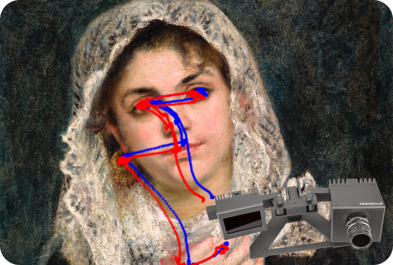
Introduction to Eye Tracking with the TRACKPixx3. Retrieved [Month, Day, Year], from https://vpixx.com/vocal/intro-to-eye-tracking/